
Discrete Fourier transform
Did you know...
SOS Children made this Wikipedia selection alongside other schools resources. With SOS Children you can choose to sponsor children in over a hundred countries
| Fourier transforms |
|---|
| Continuous Fourier transform |
| Fourier series |
| Discrete-time Fourier transform |
| Discrete Fourier transform |
|
|
|
|
In mathematics, the discrete Fourier transform (DFT) is one of the specific forms of Fourier analysis. As such, it transforms one function into another, which is called the frequency domain representation, or simply the DFT, of the original function (which is often a function in the time domain). But the DFT requires an input function that is discrete and whose non-zero values have a limited (finite) duration. Such inputs are often created by sampling a continuous function, like a person's voice. And unlike the discrete-time Fourier transform (DTFT), it only evaluates enough frequency components to reconstruct the finite segment that was analyzed. Its inverse transform cannot reproduce the entire time domain, unless the input happens to be periodic (forever). Therefore it is often said that the DFT is a transform for Fourier analysis of finite-domain discrete-time functions. The sinusoidal basis functions of the decomposition have the same properties.
Since the input function is a finite sequence of real or complex numbers, the DFT is ideal for processing information stored in computers. In particular, the DFT is widely employed in signal processing and related fields to analyze the frequencies contained in a sampled signal, to solve partial differential equations, and to perform other operations such as convolutions. The DFT can be computed efficiently in practice using a fast Fourier transform (FFT) algorithm.
Since FFT algorithms are so commonly employed to compute the DFT, the two terms are often used interchangeably in colloquial settings, although there is a clear distinction: "DFT" refers to a mathematical transformation, regardless of how it is computed, while "FFT" refers to any one of several efficient algorithms for the DFT. This distinction is further blurred, however, by the synonym finite Fourier transform for the DFT, which apparently predates the term "fast Fourier transform" (Cooley et al., 1969) but has the same initialism.
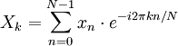
Definition
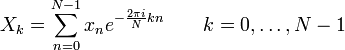
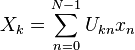
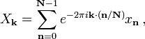
The sequence of N complex numbers x0, ..., xN−1 is transformed into the sequence of N complex numbers X0, ..., XN−1 by the DFT according to the formula:
where  is a primitive N'th root of unity.
The transform is sometimes denoted by the symbol  , as in
  or
or  or
or  .
.
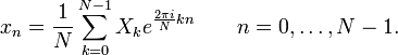
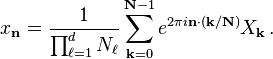
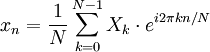
The inverse discrete Fourier transform (IDFT) is given by
A simple description of these equations is that the complex numbers  represent the amplitude and phase of the different sinusoidal components of the input "signal"
  . The DFT computes the from the , while the IDFT shows how to compute the as a sum of sinusoidal components
 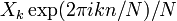 with frequency
  cycles per sample. By writing the equations in this form, we are making extensive use of Euler's formula to express sinusoids in terms of complex exponentials, which are much easier to manipulate. (In the same way, by writing in polar form, we immediately obtain the sinusoid amplitude from
  and the phase from the complex argument.) An important subtlety of this representation, aliasing, is discussed below.
Note that the normalization factor multiplying the DFT and IDFT (here 1 and 1/N) and the signs of the exponents are merely conventions, and differ in some treatments. The only requirements of these conventions are that the DFT and IDFT have opposite-sign exponents and that the product of their normalization factors be 1/N. A normalization of  for both the DFT and IDFT makes the transforms unitary, which has some theoretical advantages, but it is often more practical in numerical computation to perform the scaling all at once as above (and a unit scaling can be convenient in other ways).
(The convention of a negative sign in the exponent is often convenient because it means that is the amplitude of a "positive frequency"  . Equivalently, the DFT is often thought of as a matched filter: when looking for a frequency of +1, one correlates the incoming signal with a frequency of −1.)
In the following discussion the terms "sequence" and "vector" will be considered interchangeable.
Properties
Completeness
The discrete Fourier transform is an invertible, linear transformation
with  denoting the set of complex numbers. In other words, for any N > 0, an N-dimensional complex vector has a DFT and an IDFT which are in turn N-dimensional complex vectors.
Orthogonality
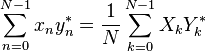
The vectors  form an orthogonal basis over the set of N-dimensional complex vectors:
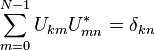
where  is the Kronecker delta. This orthogonality condition can be used to derive the formula for the IDFT from the definition of the DFT, and is equivalent to the unitarity property below.
The Plancherel theorem and Parseval's theorem
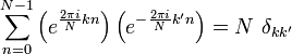
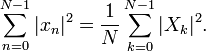
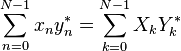
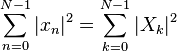
If Xk and Yk are the DFTs of xn and yn respectively then the Plancherel theorem states:
where the star denotes complex conjugation. Parseval's theorem is a special case of the Plancherel theorem and states:
These theorems are also equivalent to the unitary condition below.
Periodicity
If the expression that defines the DFT is evaluated for all integers  instead of just for
  , then the resulting infinite sequence is a periodic extension of the DFT, periodic with period N.
The periodicity can be shown directly from the definition:

where we have used the fact that  . In the same way it can be shown that the IDFT formula leads to a periodic extension.
The shift theorem
Multiplying by a linear phase  for some integer
  corresponds to a circular shift of the output : is replaced by
  , where the subscript is interpreted modulo
  (i.e., periodically). Similarly, a circular shift of the input corresponds to multiplying the output by a linear phase. Mathematically, if
  represents the vector x then
- if
- then
- and
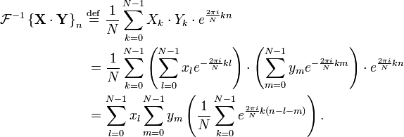
Circular convolution theorem and cross-correlation theorem
The convolution theorem for the continuous and discrete time Fourier transforms indicates that a convolution of two infinite sequences can be obtained as the inverse transform of the product of the individual transforms. With sequences and transforms of length N, a circularity arises:
The quantity in parentheses is 0 for all values of except those of the form  , where
  is any integer. At those values, it is 1. It can therefore be replaced by an infinite sum of Kronecker delta functions, and we continue accordingly. Note that we can also extend the limits of to infinity, with the understanding that the
  and
and  sequences are defined as 0 outside [0,N-1]:
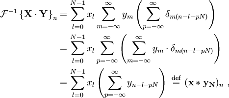
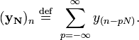
which is the convolution of the  sequence with a periodically extended
  sequence defined by:
Similarly, it can be shown that:
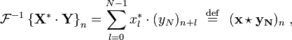
which is the cross-correlation of and 
A direct evaluation of the convolution or correlation summation, above, requires  operations. An indirect method, using transforms, can take advantage of the
  efficiency of the fast Fourier transform (FFT) to achieve much better performance. Furthermore, convolutions can be used to efficiently compute DFTs via Rader's FFT algorithm and Bluestein's FFT algorithm.
Methods have also been developed to use circular convolution as part of an efficient process that achieves normal (non-circular) convolution with an or sequence potentially much longer than the practical transform size (N). Two such methods are called overlap-save and overlap-add.
Trigonometric interpolation polynomial
The trigonometric interpolation polynomial
 for even ,
 for odd,
where the coefficients Xk /N are given by the DFT of xn above, satisfies the interpolation property  for
for  .
.
For even , notice that the Nyquist component 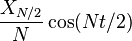 is handled specially.
This interpolation is not unique: aliasing implies that one could add N to any of the complex-sinusoid frequencies (e.g. changing  to
to  ) without changing the interpolation property, but giving different values in between the points. The choice above, however, is typical because it has two useful properties. First, it consists of sinusoids whose frequencies have the smallest possible magnitudes, and therefore minimizes the mean-square slope
  of the interpolating function. Second, if the are real numbers, then
  is real as well.
In contrast, the most obvious trigonometric interpolation polynomial is the one in which the frequencies range from 0 to  (instead of roughly
  to
to  as above), similar to the inverse DFT formula. This interpolation does not minimize the slope, and is not generally real-valued for real ; its use is a common mistake.
The unitary DFT
Another way of looking at the DFT is to note that in the above discussion, the DFT can be expressed as a Vandermonde matrix:
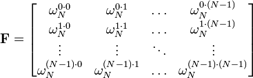
where
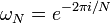
is a primitive Nth root of unity. The inverse transform is then given by the inverse of the above matrix:
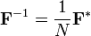
With unitary normalization constants , the DFT becomes a unitary transformation, defined by a unitary matrix:
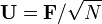

where det() is the determinant function. The determinant is the product of the eigenvalues, which are always  or
or  as described below. In a real vector space, a unitary transformation can be thought of as simply a rigid rotation of the coordinate system, and all of the properties of a rigid rotation can be found in the unitary DFT.
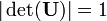
The orthogonality of the DFT is now expressed as an orthonormality condition (which arises in many areas of mathematics as described in root of unity):
If  is defined as the unitary DFT of the vector then
and the Plancherel theorem is expressed as:
If we view the DFT as just a coordinate transformation which simply specifies the components of a vector in a new coordinate system, then the above is just the statement that the dot product of two vectors is preserved under a unitary DFT transformation. For the special case  , this implies that the length of a vector is preserved as well—this is just Parseval's theorem:
Expressing the inverse DFT in terms of the DFT
A useful property of the DFT is that the inverse DFT can be easily expressed in terms of the (forward) DFT, via several well-known "tricks". (For example, in computations, it is often convenient to only implement a fast Fourier transform corresponding to one transform direction and then to get the other transform direction from the first.)
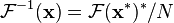
First, we can compute the inverse DFT by reversing the inputs:

(As usual, the subscripts are interpreted modulo ; thus, for  , we have
  .)
.)
Second, one can also conjugate the inputs and outputs:
Third, a variant of this conjugation trick, which is sometimes preferable because it requires no modification of the data values, involves swapping real and imaginary parts (which can be done on a computer simply by modifying pointers). Define swap() as with its real and imaginary parts swapped—that is, if  then swap() is
  . Equivalently, swap() equals
  . Then

That is, the inverse transform is the same as the forward transform with the real and imaginary parts swapped for both input and output, up to a normalization (Duhamel et al., 1988).
The conjugation trick can also be used to define a new transform, closely related to the DFT, that is involutary—that is, which is its own inverse. In particular, 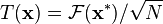 is clearly its own inverse:
 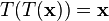 . A closely related involutary transformation (by a factor of (1+i) /√2) is
 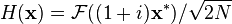 , since the
  factors in
  cancel the 2. For real inputs , the real part of
  is none other than the discrete Hartley transform, which is also involutary.
Eigenvalues and eigenvectors
The eigenvalues of the DFT matrix are simple and well-known, whereas the eigenvectors are complicated, not unique, and are the subject of ongoing research.
Consider the unitary form  defined above for the DFT of length , where
  . This matrix satisfies the equation:

This can be seen from the inverse properties above: operating twice gives the original data in reverse order, so operating four times gives back the original data and is thus the identity matrix. This means that the eigenvalues  satisfy a characteristic equation:

Therefore, the eigenvalues of are the fourth roots of unity: is +1, −1, +i, or −i.
Since there are only four distinct eigenvalues for this  matrix, they have some multiplicity. The multiplicity gives the number of linearly independent eigenvectors corresponding to each eigenvalue. (Note that there are N independent eigenvectors; a unitary matrix is never defective.)
The problem of their multiplicity was solved by McClellan and Parks (1972), although it was later shown to have been equivalent to a problem solved by Gauss (Dickinson and Steiglitz, 1982). The multiplicity depends on the value of modulo 4, and is given by the following table:
| size N | λ = +1 | λ = −1 | λ = -i | λ = +i |
|---|---|---|---|---|
| 4m | m + 1 | m | m | m − 1 |
| 4m + 1 | m + 1 | m | m | m |
| 4m + 2 | m + 1 | m + 1 | m | m |
| 4m + 3 | m + 1 | m + 1 | m + 1 | m |
Unfortunately, no simple analytical formula for the eigenvectors is known. Moreover, the eigenvectors are not unique because any linear combination of eigenvectors for the same eigenvalue is also an eigenvector for that eigenvalue. Various researchers have proposed different choices of eigenvectors, selected to satisfy useful properties like orthogonality and to have "simple" forms (e.g., McClellan and Parks, 1972; Dickinson and Steiglitz, 1982; Grünbaum, 1982; Atakishiyev and Wolf, 1997; Candan et al., 2000; Hanna et al., 2004).
The choice of eigenvectors of the DFT matrix has become important in recent years in order to define a discrete analogue of the fractional Fourier transform—the DFT matrix can be taken to fractional powers by exponentiating the eigenvalues (e.g., Rubio and Santhanam, 2005). For the continuous Fourier transform, the natural orthogonal eigenfunctions are the Hermite functions, so various discrete analogues of these have been employed as the eigenvectors of the DFT, such as the Kravchuk polynomials (Atakishiyev and Wolf, 1997). The "best" choice of eigenvectors to define a fractional discrete Fourier transform remains an open question, however.
The real-input DFT
If  are real numbers, as they often are in practical applications, then the DFT obeys the symmetry:
where the star denotes complex conjugation and the subscripts are interpreted modulo N.
Therefore, the DFT output for real inputs is half redundant, and one obtains the complete information by only looking at roughly half of the outputs  . In this case, the "DC" element
  is purely real, and for even N the "Nyquist" element
  is also real, so there are exactly N non-redundant real numbers in the first half + Nyquist element of the complex output X.
Using Euler's formula, the interpolating trigonometric polynomial can then be interpreted as a sum of sine and cosine functions.
Generalized/shifted DFT
It is possible to shift the transform sampling in time and/or frequency domain by some real shifts a and b, respectively. This is sometimes known as a generalized DFT (or GDFT), also called the shifted DFT or offset DFT, and has analogous properties to the ordinary DFT:
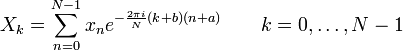
Most often, shifts of  (half a sample) are used. While the ordinary DFT corresponds to a periodic signal in both time and frequency domains,
  produces a signal that is anti-periodic in frequency domain (
 ) and vice-versa for
  . Thus, the specific case of
  is known as an odd-time odd-frequency discrete Fourier transform (or O2 DFT). Such shifted transforms are most often used for symmetric data, to represent different boundary symmetries, and for real-symmetric data they correspond to different forms of the discrete cosine and sine transforms.
Another interesting choice is  , which is called the centered DFT (or CDFT). The centered DFT has the useful property that, when is a multiple of four, all four of its eigenvalues (see above) have equal multiplicities (Rubio and Santhanam, 2005).
The discrete Fourier transform can be viewed as a special case of the z-transform, evaluated on the unit circle in the complex plane; more general z-transforms correspond to complex shifts a and b above.
Multidimensional DFT
The ordinary DFT computes the transform of a "one-dimensional" dataset: a sequence (or array) that is a function of one discrete variable  . More generally, one can define the multidimensional DFT of a multidimensional array
  that is a function of
  discrete variables
  for
for  in
in  :
:
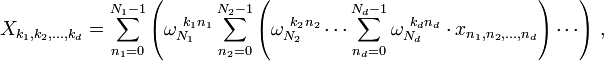
where  as above and the output indices run from
  . This is more compactly expressed in vector notation, where we define
  and
and  as -dimensional vectors of indices from 0 to
  , which we define as
  :
:
where the division  is defined as
  to be performed element-wise, and the sum denotes the set of nested summations above.
The inverse of the multi-dimensional DFT is, analogous to the one-dimensional case, given by:
The multidimensional DFT has a simple interpretation. Just as the one-dimensional DFT expresses the input as a superposition of sinusoids, the multidimensional DFT expresses the input as a superposition of plane waves, or sinusoids oscillating along the direction  in space and having amplitude
  . Such a decomposition is of great importance for everything from digital image processing (d = 2) to solving partial differential equations in three dimensions (d = 3) by breaking the solution up into plane waves.
Computationally, the multidimensional DFT is simply the composition of a sequence of one-dimensional DFTs along each dimension. For example, in the two-dimensional case  one can first compute the
  independent DFTs of the rows (i.e., along
  ) to form a new array
  , and then compute the
  independent DFTs of along the columns (along
  ) to form the final result
  . Or, one can transform the columns and then the rows—the order is immaterial because the nested summations above commute.
Because of this, given a way to compute a one-dimensional DFT (e.g. an ordinary one-dimensional FFT algorithm), one immediately has a way to efficiently compute the multidimensional DFT. This is known as a row-column algorithm, although there are also intrinsically multidimensional FFT algorithms.
The real-input multidimensional DFT
If the inputs are real numbers, as they often are in practical applications, then the DFT outputs have a conjugate symmetry similar to the one-dimensional case above:

where the star denotes complex conjugation and the -th subscript is interpreted modulo  (for
(for 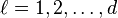 ).
).
Applications
The DFT has seen wide usage across a large number of fields; we only sketch a few examples below (see also the references at the end). All applications of the DFT depend crucially on the availability of a fast algorithm to compute discrete Fourier transforms and their inverses, a fast Fourier transform.
Spectral analysis
When the DFT is used for spectral analysis, the  sequence usually represents a finite set of uniformly-spaced time-samples of some signal
  , where t represents time. The conversion from continuous time to samples (discrete-time) changes the underlying Fourier transform of x(t) into a discrete-time Fourier transform (DTFT), which generally entails a type of distortion called aliasing. Choice of an appropriate sample-rate (see Nyquist frequency) is the key to minimizing that distortion. Similarly, the conversion from a very long (or infinite) sequence to a manageable size entails a type of distortion called leakage, which is manifested as a loss of detail (aka resolution) in the DTFT. Choice of an appropriate sub-sequence length is the primary key to minimizing that effect. When the available data (and time to process it) is more than the amount needed to attain the desired frequency resolution, a standard technique is to perform multiple DFTs, for example to create a spectrogram. If the desired result is a power spectrum and noise or randomness is present in the data, averaging the magnitude components of the multiple DFTs is a useful procedure to reduce the variance of the spectrum (also called a periodogram in this context); two examples of such techniques are the Welch method and the Bartlett method.
A final source of distortion (or perhaps illusion) is the DFT itself, because it is just a discrete sampling of the DTFT, which is a function of a continuous frequency domain. That can be mitigated by increasing the resolution of the DFT. That procedure is illustrated in the discrete-time Fourier transform article.
- The procedure is sometimes referred to as zero-padding, which is a particular implementation used in conjunction with the fast Fourier transform (FFT) algorithm. The inefficiency of performing multiplications and additions with zero-valued "samples" is more than offset by the inherent efficiency of the FFT.
- As already noted, leakage imposes a limit on the inherent resolution of the DTFT. So there is a practical limit to the benefit that can be obtained from a fine-grained DFT.
Data compression
The field of digital signal processing relies heavily on operations in the frequency domain (i.e. on the Fourier transform). For example, several lossy image and sound compression methods employ the discrete Fourier transform: the signal is cut into short segments, each is transformed, and then the Fourier coefficients of high frequencies, which are assumed to be unnoticeable, are discarded. The decompressor computes the inverse transform based on this reduced number of Fourier coefficients. (Compression applications often use a specialized form of the DFT, the discrete cosine transform or sometimes the modified discrete cosine transform.)
Partial differential equations
Discrete Fourier transforms are often used to solve partial differential equations, where again the DFT is used as an approximation for the Fourier series (which is recovered in the limit of infinite N). The advantage of this approach is that it expands the signal in complex exponentials einx, which are eigenfunctions of differentiation: d/dx einx = in einx. Thus, in the Fourier representation, differentiation is simple—we just multiply by i n. A linear differential equation with constant coefficients is transformed into an easily solvable algebraic equation. One then uses the inverse DFT to transform the result back into the ordinary spatial representation. Such an approach is called a spectral method.
Polynomial multiplication
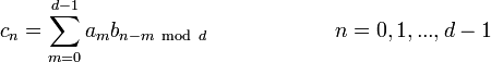
Suppose we wish to compute the polynomial product c(x) = a(x) · b(x). The ordinary product expression for the coefficients of c involves a linear (acyclic) convolution, where indices do not "wrap around." This can be rewritten as a cyclic convolution by taking the coefficient vectors for a(x) and b(x) with constant term first, then appending zeros so that the resultant coefficient vectors a and b have dimension d > deg(a(x)) + deg(b(x)). Then,

Where c is the vector of coefficients for c(x), and the convolution operator  is defined so
But convolution becomes multiplication under the DFT:
Here the vector product is taken elementwise. Thus the coefficients of the product polynomial c(x) are just the terms 0, ..., deg(a(x)) + deg(b(x)) of the coefficient vector
With a Fast Fourier transform, the resulting algorithm takes O (N log N) arithmetic operations. Due to its simplicity and speed, the Cooley-Tukey FFT algorithm, which is limited to composite sizes, is often chosen for the transform operation. In this case, d should be chosen as the smallest integer greater than the sum of the input polynomial degrees that is factorizable into small prime factors (e.g. 2, 3, and 5, depending upon the FFT implementation).
Multiplication of large integers
The fastest known algorithms for the multiplication of very large integers use the polynomial multiplication method outlined above. Integers can be treated as the value of a polynomial evaluated specifically at the number base, with the coefficients of the polynomial corresponding to the digits in that base. After polynomial multiplication, a relatively low-complexity carry-propagation step completes the multiplication.
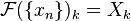
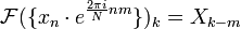
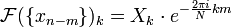
Some discrete Fourier transform pairs
 |
 |
Note |
|---|---|---|
 |
 |
Shift theorem |
 |
 |
|
 |
 |
Real DFT |
 |
 |
|
 |
 |
Derivation as Fourier series
The DFT can be derived as a truncation of the Fourier series of a periodic sequence of impulses.
DFT over fields other than the complex numbers
Many of the properties of the DFT only depend on the fact that  is a primitive root of unity, sometimes denoted
  or
or  (so that
  ). Such properties include the completeness, orthogonality, Plancherel/Parseval, periodicity, shift, convolution, and unitarity properties above, as well as many FFT algorithms. For this reason, the discrete Fourier transform can be defined by using roots of unity in fields other than the complex numbers; for more information, see discrete Fourier transform (general).